Geerts_2023_PBPK_QSP_SBML_Model

Model Details

This document provides detailed technical information about the Geerts model implementation, including module structure, methodology, and key technical considerations.

Table of Contents

• Model Architecture
• Module Structure
• ODE to Reactions Translation
• Key Technical Components
• Parameter Management
• Model Generation and Execution

Model Architecture

The model is implemented using a modular architecture where individual biological processes are separated into distinct modules. This approach provides several advantages:

• Modularity: Each biological process can be developed and validated independently
• Flexibility: Components can be easily modified or replaced
• Maintainability: Clear separation of concerns makes debugging easier
• Reusability: Modules can be reused in different model configurations

Multiple Implementation Approaches

1. SBML-based Implementation: Uses Systems Biology Markup Language for model representation
2. Direct ODE Implementation: JAX-based ODE system directly translated from published equations

Model Structure

The model is organized into several modules, each responsible for specific aspects of the system:

QSP Components (Amyloid Beta Kinetics)

1. AB_production.py
   • Models amyloid precursor protein (APP) processing and Aβ production
   • Includes APP production, C99 fragment formation, Aβ40 and Aβ42 monomer production
   • Accounts for IDE-mediated clearance of Aβ monomers
2. Geerts_dimer.py
   • Models Aβ dimer formation and dynamics
   • Includes dimer formation from monomers, dissociation back to monomers
   • Accounts for plaque-catalyzed dimer formation and antibody binding
3. Geerts_Oligomer_3_12.py
   • Models small Aβ oligomer formation and dynamics (3-12mers)
   • Includes oligomer formation from smaller species and monomers
   • Accounts for oligomer dissociation, plaque formation, and antibody binding
   • Includes antibody binding and microglia-mediated clearance
4. Geerts_Oligomer_13_16.py
   • Models medium Aβ oligomer formation and dynamics (13-16mers)
   • Similar processes to small oligomers but for larger species
   • Includes transition to plaque formation
   • Includes antibody binding and microglia-mediated clearance
5. Geerts_Fibril_17_18.py
   • Models small Aβ fibril formation and dynamics (17-18mers)
   • Includes fibril formation from oligomers and monomers
   • Accounts for fibril dissociation and plaque formation
   • Includes antibody binding and microglia-mediated clearance
6. Geerts_Fibril_19_24.py
   • Models large Aβ fibril (19-24mers) and plaque formation and dynamics
   • Similar processes to small fibrils but for larger species
   • Includes final transition to plaque formation
   • Includes antibody binding and microglia-mediated clearance

PBPK Components (Antibody Distribution)

1. Geerts_PBPK_mAb.py
   • Models monoclonal antibody (mAb) pharmacokinetics in the brain
   • Includes antibody distribution across blood-brain barrier (BBB)
   • Accounts for FcRn-mediated antibody recycling
   • Includes antibody binding to Aβ species and clearance mechanisms
2. Geerts_PBPK_monomers.py
   • Models Aβ monomer pharmacokinetics in the brain
   • Could be considered part of the QSP model, but this is very Physiology Based
   • Includes monomer distribution across BBB and blood-CSF barrier
   • Accounts for monomer clearance through various pathways
   • Includes monomer production and degradation
   • Includes monomer antibody binding reactions
3. Geerts_PVS_ARIA.py
   • Models perivascular space (PVS) dynamics
   • ARIA is not implemented yet
   • Includes perivascular space fluid flow and transport
   • Includes clearance of Aβ through the glymphatic system
   • Models antibody and Aβ transport between PVS and ISF
4. geerts_microglia.py
   • Models microglia-mediated clearance of Aβ species
   • Includes microglia dependent clearance of bound species
   • Accounts for high and low activity states
   • Includes antibody-dependent microglial activation
   • Models microglia cell population dynamics

ODE to Reactions Translation

A key aspect of this implementation is the translation from published ordinary differential equations (ODEs) to reaction-based SBML format. This translation required several important considerations:

Mass Units Conversion

The original Geerts model uses concentration units (nM), but SBML reactions work best with mass units. Our implementation:

• Converts all concentrations to mass units using compartment volumes
• Maintains consistency across all reactions and rate constants
• Validates the conversion by comparing with direct ODE implementation

Reaction Network Construction

Each ODE term is translated into corresponding reactions:

• Production terms become synthesis reactions
• Degradation terms become degradation reactions
• Transport terms become transport reactions between compartments
• Binding interactions become association/dissociation reaction pairs
• Some Rate Rules / Assignment Rules are still required for time dependent terms
  • Microglia Cell Count
  • IDE clearance rate
  • Antibody Dosing forcing function

Rate Constant Handling

Rate constants are carefully managed to ensure:

• Proper units (converted from concentration-based to mass-based rates)
• Appropriate scaling for compartment volumes

Key Technical Components

Rate Constant Extrapolation

The model uses sophisticated rate extrapolation implemented in K_rates_extrapolate.py:

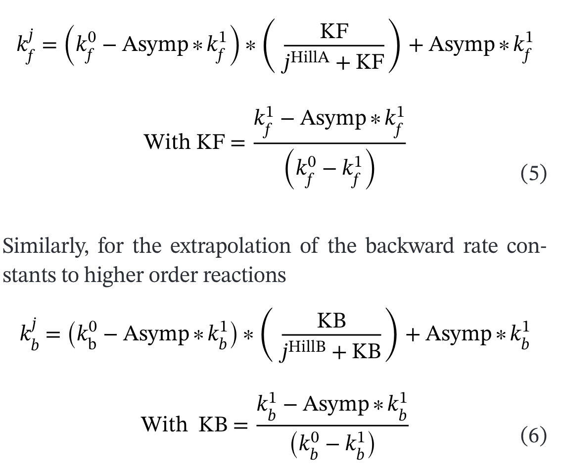
Forward and Backward rate constants for higher order aggregates extrapolated from experimentally determined low order rates. This file also creates the 𝐹𝑖𝑏𝐹𝑜𝑟𝐴𝑗 rates used for direct formation of Plaques from higher order oligomers. This section of the model has minimal information in the supplement and has required significant assumptions to be made.

Key Features:

• Uses experimentally determined rates for small oligomers as anchor points
• Handles Aβ40 and Aβ42 separately with different aggregation propensities
• Defines $\text{FibForAj}$ rates as $K_{\text{O13_Plaque_42}} = K_{\text{O13_O14_42}} \times \text{Baseline_AB42_Oligomer_Fibril_Plaque}$ using Oligomer_13 as an example
• Note: Backward rates are not provided in the original supplement and are copied from referenced paper Garai 2013
• Note: Found issues with Garai Rates including one issue in publication itself and another discrepancy between rate in Geerts and published rate
  • Garai et al. 2013 Figure 7 fails for published value of dimer to trimer rate for Abeta 42: k+23 (kf1 in Geerts) = 38 (M⁻¹s⁻¹), but is reproducible with k+23 = 380 (M⁻¹s⁻¹)
  • Geerts TableS2 cites Garai for kf0 and kf1, but is missing kb0 and kb1
  • Geerts TableS2 has kf0 ABeta 42 = 0.0003564 nM/h = 9.9 (M⁻¹s⁻¹) when Garai has 9.9 (M⁻¹s⁻¹) × 10²

The full rate extrapolation is shown below with oligomer size on the x-axis. Notice that for Aβ42, the backward rate consistently exceeds the forward rate throughout the size range. We believe this imbalance is responsible for the overabundance of monomers and failure to aggregate effectively.

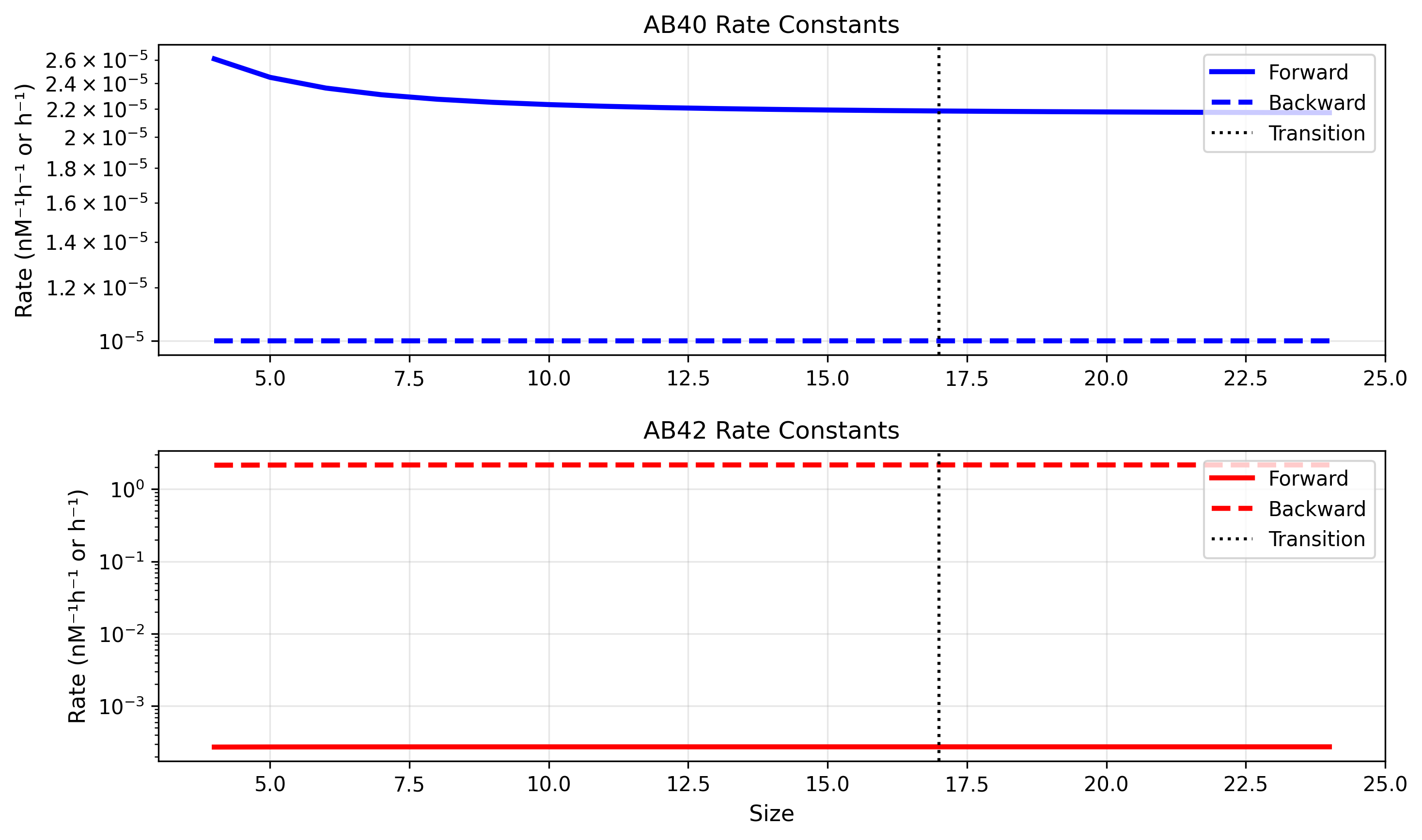
Through sensitivity analysis of the low-order backward rates omitted from the Geerts supplement, we determined that the reported values for Aβ42 in Garai 2013 are likely much higher than physiologically realistic. The table below compares the original Garai values with our adjusted parameters:

Parameter	Garai 2013	Our Model
k_O2_M_42	45.72	45.72
k_O3_O2_42	1.08	1E-05

We maintained the dimer-to-monomer rate at the original value but reduced the trimer-to-dimer rate to the reported cutoff threshold for backward rates. This deviation from the original Garai rates was essential to capture age-dependent aggregation behavior, which is crucial for this model’s physiological relevance.

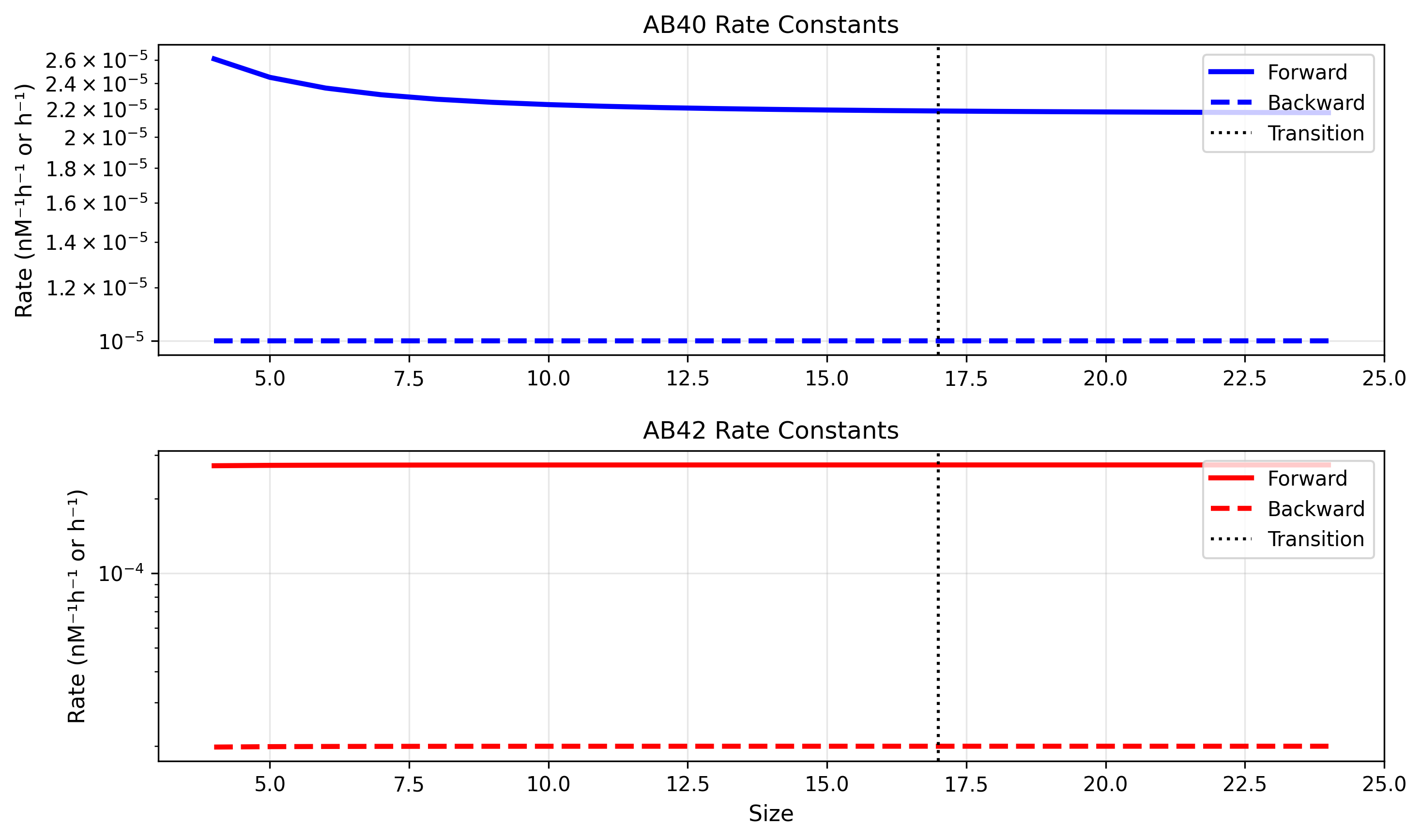
With these adjustments, the forward rate now exceeds the backward rate for both Aβ40 and Aβ42 species, enabling proper aggregation dynamics.

• Note Similar bahvior can be reacted by lowering k_O2_M_42 or increasing low order forwarded rates.

IDE Clearance Decline with Age

The model implements age-dependent decline in insulin-degrading enzyme (IDE) clearance in the equation for monomer dynamics:

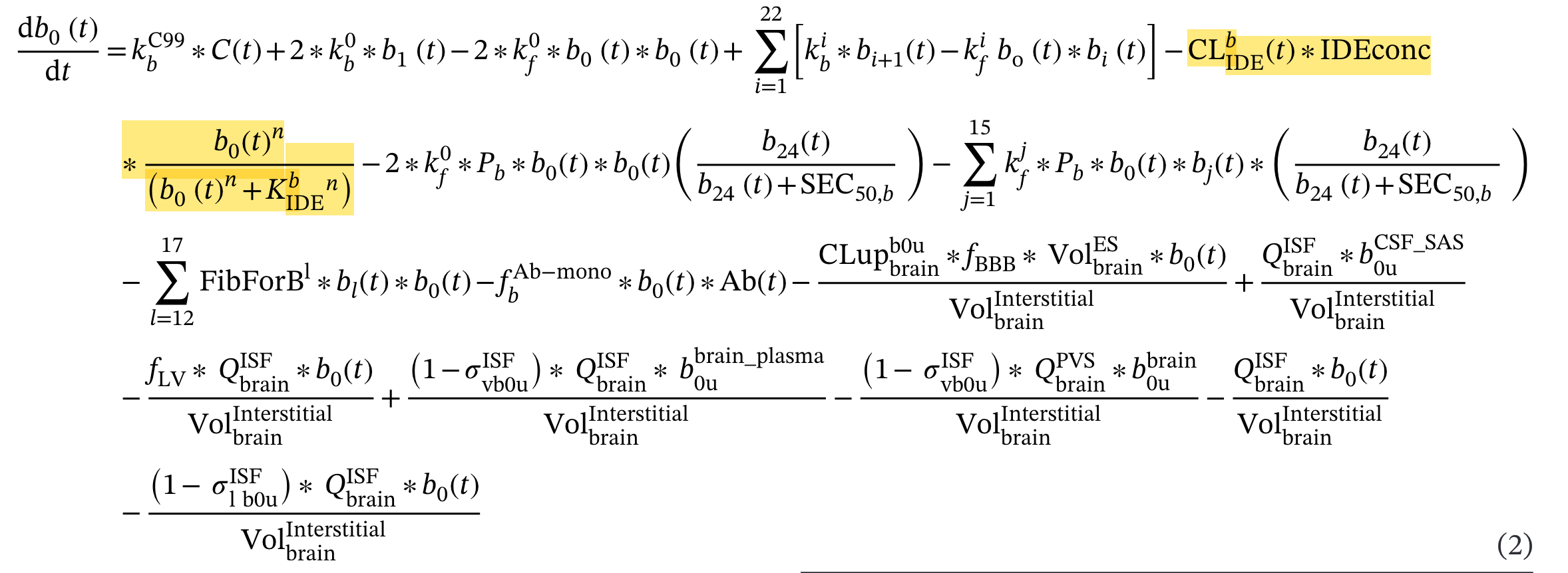
The clearance term has its own time-dependent behavior

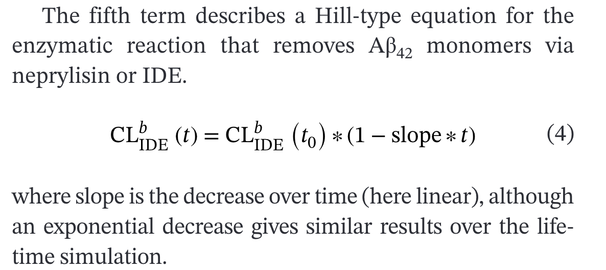
Important Note: This age-dependent decline is mentioned in the main publication but the specific equation and parameters are not provided in Supplementary Table 2.

# This term is represented here as it is in TableS2 without the slope or time dependent behavior

 -(IDE_conc * AB42_IDE_Kcat_lin * ((AB42_Monomer * Unit_removal_1)^AB42_IDE_Hill / ((AB42_Monomer * Unit_removal_1)^AB42_IDE_Hill 

No equation is given to show how clearance changes with age so we chose to implement one based on the IDE equation from the main paper. A linear slope was unavailable in the supplement so we chose to use the published exponential decline rate.

Individual Oligomer Tracking

The model tracks individual oligomer species (2-mers through 24-mers) rather than using averaged pools. This provides:

• Detailed Species Resolution: Each oligomer size has distinct kinetic properties
• Size-Dependent Behavior: Aggregation and clearance rates vary with oligomer size
• Validation Capability: Individual species can be compared with experimental data
• Mechanistic Insight: Understanding of aggregation cascade progression

Microglia Dynamics with Dosing

Microglia activation responds to antibody-bound amyloid:

Results for Gantenerumab 3-year study with dosing every 4 weeks for 1.5 years

Dynamic Features:

• Baseline activation level in absence of treatment
• Enhanced activation in response to antibody-bound Aβ
• Cell population dynamics
• Clearance capacity modulation

Parameter Management

Parameter Documentation Structure

Parameters are stored in parameters/PK_Geerts.csv with comprehensive documentation:

Column	Description
name	Parameter identifier used in code
value	Numerical value
units	Physical units
Sup_Name	Original name from Geerts supplement
Source	Literature reference
Validated	Binary flag (1 = personally verified)
Notes	Additional comments

Parameter Validation Status

The model includes a systematic parameter validation approach:

• Validated Parameters (Validated = 1): Personally verified against literature
• Unvalidated Parameters (Validated = 0): Require further verification
• Source Traceability: Each parameter linked to specific literature reference
• Units Standardization: All parameters use consistent unit systems

Model Generation and Execution

Generation Process

1. Module Combination: Combined_Master_Model.py merges all modules
2. SBML Export: Generated model saved as XML in generated/sbml/
3. JAX Conversion: SBML converted to JAX format using sbml_to_ode_jax
4. Validation: Cross-validation with direct ODE implementation

Execution Schemes

Multi-Dose Simulation

1. Generate combined SBML model
2. Convert to JAX format  
3. Run steady-state simulation (no dose)
4. Use steady-state as initial condition
5. Apply dosing schedule
6. Generate comprehensive outputs

No-Dose Simulation

1. Generate model without dosing components
2. Run long-term simulation (20-100 years)
3. Focus on natural Aβ aggregation dynamics
4. Useful for parameter sensitivity analysis

Solver Configuration

The model uses sophisticated ODE solvers:

• Primary Solver: Tsit5 (5th order Runge-Kutta)
• JAX Integration: Leverages JAX for automatic differentiation
• Diffrax Backend: Modern ODE solving with advanced numerical methods
• CVODE: Used in Tellurium

Technical Limitations and Considerations

Current Limitations

1. Aggregation Dynamics: Investigating discrepancies in Aβ aggregation behavior
2. Parameter Uncertainty: Some parameters lack direct experimental validation
3. Computational Cost: Full model has significant runtime for long simulations
4. Dosing in Tellurium: Currently the use of Tellurium helps reduce runtime significantly for our no dose simulations, but we are unable to get the dosing scheduale to work using this tool.

Ongoing Validation

• Parameter sensitivity analysis using Tellurium framework
• Comparison with published experimental data
• Investigation of aggregation pathway parameters